Validation

Benchmarks comparing MoCSI against analytical solutions, other published thermophysical models, and radiosity reference cases.

Validation of solver and boundary conditions

Comparison with analytical solution

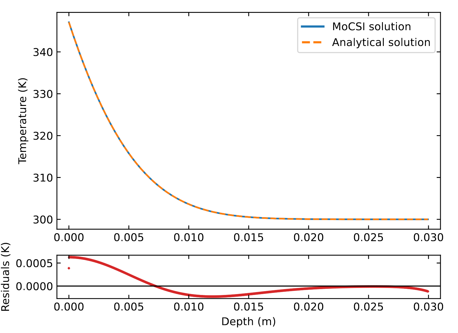
We compared the simulated temperatures by MoCSI with the analytical solution given in Incropera et al. (1996, eq. 5.59) for a semi-infinite domain with no flux at the bottom and a constant heat flux at the top:

\[ T(x,t)=T_{\mathrm{initial}} +\frac{q_0}{k}\left( 2\sqrt{\frac{\alpha t}{\pi}}\, \exp\left(-\frac{x^{2}}{4\alpha t}\right) - x\,\operatorname{erfc}\left(\frac{x}{2\sqrt{\alpha t}}\right) \right) \]

with the starting temperature of the entire domain \(T_{\text{initial}}\), the constant surface heat flux \(q_0\), the thermal diffusivity \(\alpha = \frac{k}{c_p \, \rho}\) and the complementary error function \(\text{erfc}\left(x\right)\). The temperature and the residuals are shown below. The residuals do not exceed 0.001 K.

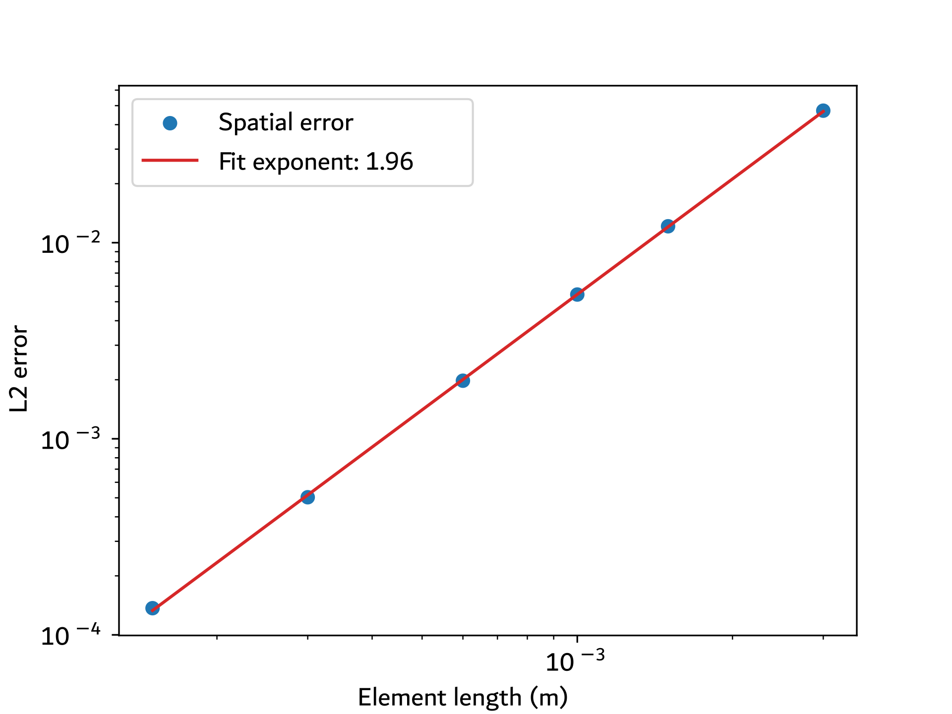
We also observe the expected order of convergence, i.e., \(O(\Delta t)\) (first order) for the temporal step size

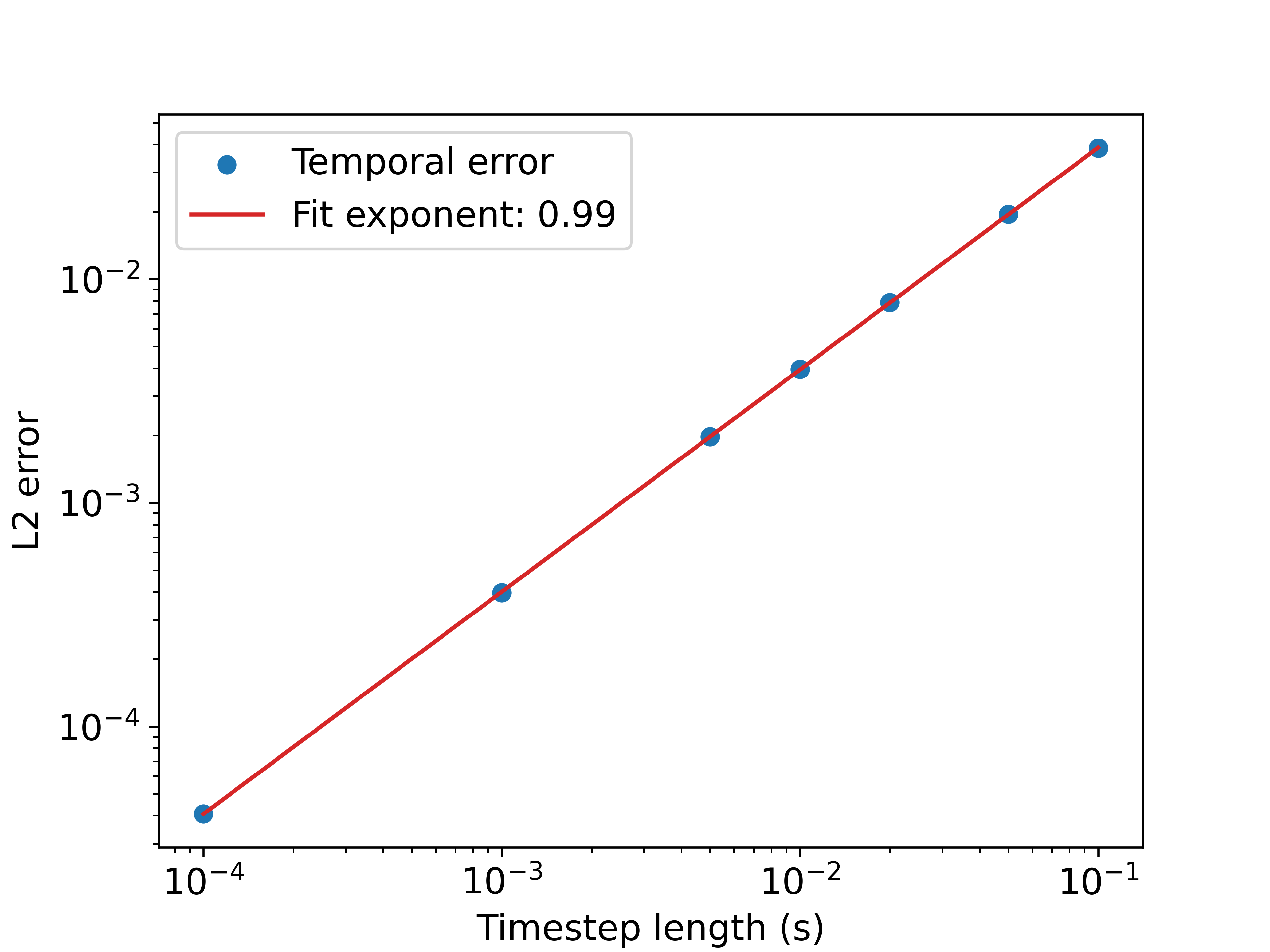
and \(O(\Delta x^2)\) (second order) for the spatial step size.

Comparison with existing thermophysical models

Schörghofer model (1DTM)

We compared MoCSI to the 1DTM developed by Norbert Schörghofer (Schörghofer & Khatiwala, 2024). The simulated temperatures by the 1DTM and MoCSI and their residuals are shown for different local times below.

We see an excellent agreement, i.e., \(\Delta T_{\text{max}} < 1\) K or \(\Delta T_{\text{max, rel}} < 1\%\), during both day and night time between 1DTM and MoCSI. There is a notable difference between the models during sunrise and sunset with differences up to 5.8 K or 5.6%. This is expected, as the Voltera predictor used in Schörghofer & Khatiwala (2024) is not implemented in MoCSI. We refer to Schuckart et al. (2026) for further details.

Hayne model (heat1d)

Additionally, we compared MoCSI to the heat1d thermal model by Hayne et al. (2017). The simulated temperatures by the heat1d model and MoCSI and their residuals are shown for different local times below.

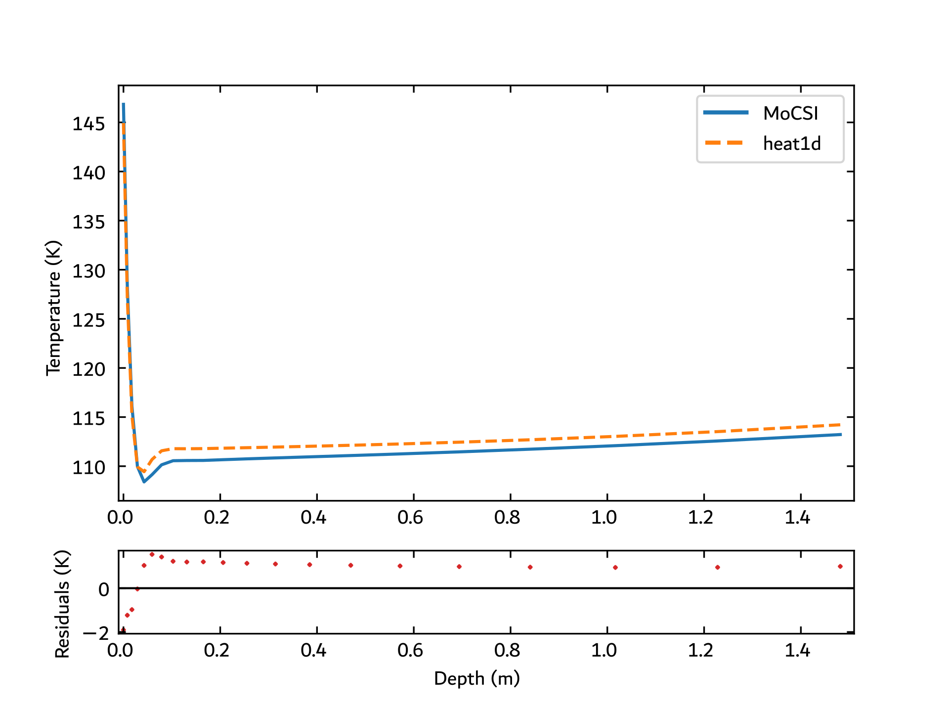
The differences between MoCSI and heat1d are on the order of \(\Delta T_{\text{max}} < 1\) K for the interior and \(\Delta T_{\text{max}} ≃ 1.9\) K for the upper boundary condition or \(\Delta T_{\text{max, rel}} ≃ 2.6\%\) and \(\Delta T_{\text{max, rel}} ≃ 5.0\%\) respectively. The differences for the interior points arise from two factors: the models treat the terms differently, and they evaluate the depth-dependent thermal properties at different positions within the grid. The differences for the surface temperature due to differences in the treatment of the upper boundary condition are more complex. We refer to Schuckart et al. (2026) for further details.

Validation of radiosity module

To verify our implementation of the viewfactor calculation and energy calculation, we compared our results for a spherical crater with no sub-surface heat transport to the analytical solution described by Ingersoll et al. (1992) as can be seen in the image below. Due to the finite number of facets, the fluctuations of the values in the shadowed region in the crater are to be expected. The crater has been generated with the publicly available code by Potter et al. 2023.

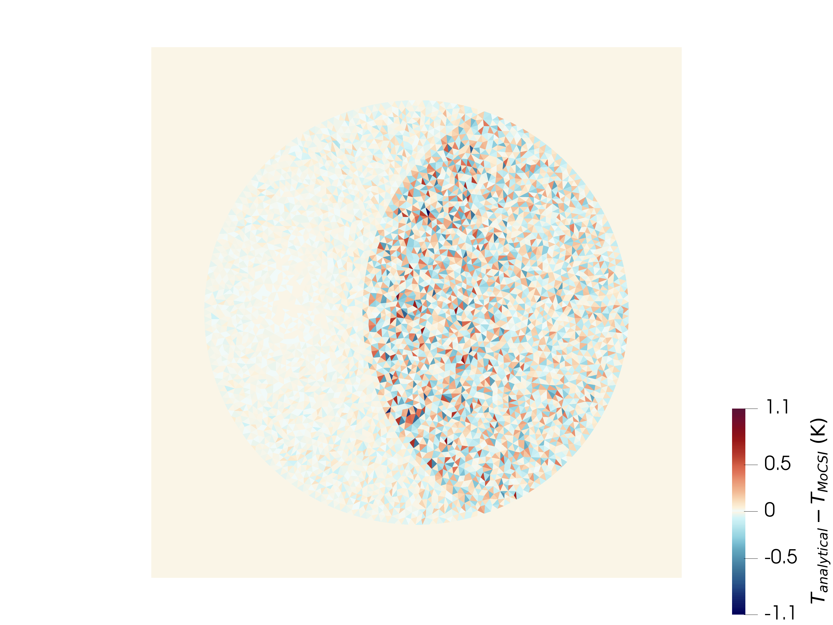
For more details on the comparison please check out the MoCSI simulation examples.